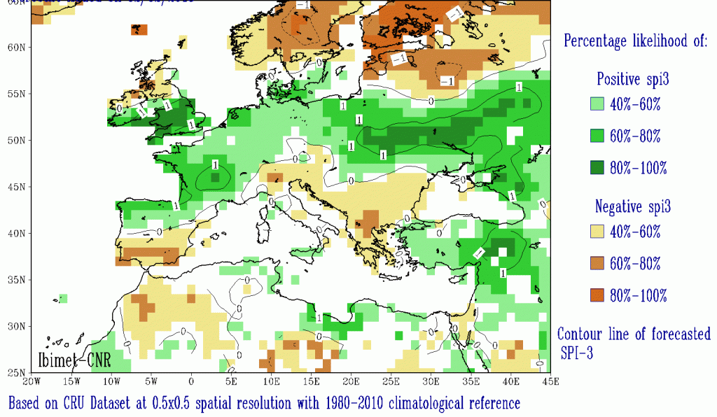
The forecasting system is based on an empirical approach to predict meteorological drought using the SPI 3 index, few months in advance from large scale observed climate indices.

SPI 3 seasonal forecast valid for February-March-April 2018. Colors scale indicates the probability of occurrence of a wet (green) or dry (yellow-orange) period.
Estimating Drought Correlation with large Scale Drivers
A physically-based statistical approach:
a Multivariate Regression model (MR) to predict future anomalies.
- In the first phase, we use a double step procedure to select the best MR model in terms of predictive performance, i.e. which are the large scale atmospheric drivers (and their lags) to use as predictors for SPI-3.
- In the second phase, we estimate the value of MR parameters that reproduce the linear relation between SPI-3 and each driver selected at 1).
- In the third phase, we use the parameter estimates obtained at 2) to predict future SPI-3 anomaly.
The SPI-3 dependent variable of the MR model is calculated using global CRU rainfall dataset (from 1901 to the present). For the SPI computation, which is done by using the “SPEI – R Package“, the Pearson III distribution and the period 1961-2010 are used for standardizing the variable to a Gaussian distribution with zero mean and standard deviation of one.
Predictors are selected among observed atmospheric and oceanic climatic indices according to the list below, then they are centered and standardized by using the overall mean and standard deviation, respectively.
The de-trending procedure is applied by monthly sub-setting each time series since an MR model is built for each forecast month.
Furthermore, a maximum of five months leading up to the forecast SPI-3 are set for each predictor to be included in the design matrix of the regressors.
For example, the design matrix of the SPI-3 model of March is composed of the predictors’ timeseries from October to February, since the SPI-3 of March is computed by using the precipitation of March, April and May.
The de-trending procedure is based on a local nonparametric regression and is applied to the dependent variable as well. Finally, 12 design matrices with 43 observations, that is, monthly values of the 1974–2015 time series, and 13∗5 predictors, are set, being 13 indices and five leading time steps.
Then, a procedure of deletion has been applied in order to address the well-known issue of multi-collinearity in MR models by eliminating linear combinations as well as high correlation between explanatory variables.
From this filtered design matrix, a double-steps procedure is applied to select the best model in terms of predictive performance:
- find the eight best models for each group of one up to 12 predictors according to the adjusted R2 index;
- find the best model among those identified at (1) by means of 10-fold cross-validation criterion and RMSE index. The entire procedure has been carried out at each grid cell of the spatial domain.
Climatic indices identified as possible predictors
Model evaluation and predictive performance
Summary of the results
An evaluation of the predictive performance of the best model for each SPI-3 is done, summarizing the results obtained in each grid cell. The great number of values above 0.50 reveals generally a good model definition. This behavior is more pronounced during winter season, when drought can be more critical. Lower performance was identified in summer period, when dryness events are common and thus have weaker impacts.
Evaluation
Predictive Performance
About the summary of the results obtained in each grid cell
signif 0.05 and signif 0.10 represent the percentage of predictors in the best model that result individually significant at level α = 0.05 and α = 0.10 of the t-test, respectively. adjR² and RMSE range is the minimum and maximum value obtained throughout the spatial domain; the SPI range is the minimum and maximum value observed.


