
Drought Scan (DS) is a framework designed to provide a clear, coherent, and scalable interpretation of drought conditions at river-basin scale.
Conceived as an operational climate service, DS is tailored for users with different profiles – technicians, researchers, water managers, irrigation consortia, and public authorities – who require tools that are immediately interpretable yet scientifically robust.
The system is based on the analysis of cumulative monthly precipitation (P) and, where available, monthly mean river discharge (Q) at the basin closing section.
These variables, representing the input and output of a simplified hydrological balance, allow drought events to be contextualized along the full meteoro-hydrological continuum, enabling the assessment of impact propagation and the modulating influence of both physical and anthropogenic factors (e.g., abstractions, reservoirs, return flows, etc.).

From an operational perspective, Drought Scan enables to:
- reconstruct and characterize major historical droughts affecting the basin
- identify the intensity, duration, and precipitation deficit using objective and reproducible metrics
- have a synthetic and flexible monitoring system based on standardized, comparable indicators
- estimate river discharge even in the presence of observational gaps, provided that a historical series is available for calibration
- analyze hydrological memory of the system
- distinguish natural discharge deficits from those amplified by anthropogenic pressures
- detect multi-year precipitation cycles and determine the current phase of the system
- provide seasonal predictions of rainfall surplus/deficit over a 1 to 6-month horizon
DS is built upon monthly standardized precipitation and discharge indices (SPI and SQI), computed across time scales ranging from 1 to 36 months. From these multiscale series emerge the three pillars of the system
Heatmap
Synthetic multiscale index D(SPI)
CDN (Cumulative Deviation from Normal)
Heatmap
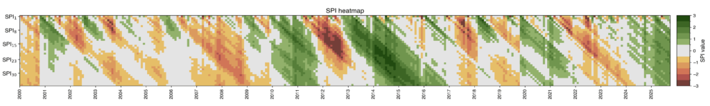
The Heatmap provides a synthetic and continuous visualisation of the historical evolution of SPI and SQI indices (when discharge data are available) across all 1 to 36 monthly time scales aggregation.
By examining the short-term scales—those of the first few months—it becomes possible to detect the onset and intensity of meteorological droughts, meaning precipitation deficits occurring over the shortest aggregation periods. Depending on their duration and severity, these “shots” can propagate to longer time scales, giving rise to prolonged and more structured drought events.
Thanks to its immediate visual clarity, the Heatmap makes it possible to identify:
- major historical droughts that triggered water crises, emergencies, or significant media attention
- intense rainfall events which, although not necessarily recovering multi-year deficits, can interrupt or temporarily ease an ongoing drought phase
- the dynamics of deficit and surplus propagation—patterns that would be impossible to detect by observing a single SPI value or a single time scale
The Heatmap, therefore, represents the starting point of the DS system: it offers an overarching view that links past conditions, the current state, and the potential future trajectories of drought within the basin.
How to read the Heatmap
- Rows: SPI values at different temporal aggregation scales (SPI1–SPI36). Each row shows how the SPI (or other SPI-like indices) evolves over time for that specific scale.
- Columns: the monthly time series under consideration.
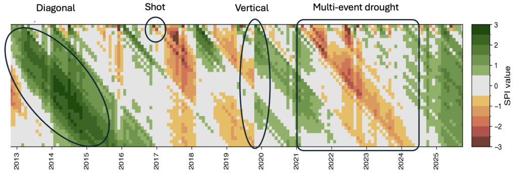
- Shot: meteorological drought episodes that emerge at the shortest time scales and that, if particularly intense, can propagate toward longer time scales, developing into prolonged droughts.
- Verticals: abrupt changes in the precipitation regime, often associated with intense rainfall events that may interrupt or ease an ongoing drought phase.
- Diagonals: indicate the temporal propagation of a drought (red diagonals) or a precipitation surplus (green diagonals).
- Multi-event droughts: short drought episodes, which may appear disconnected, can actually belong to a single continuum that evolves into a more intense and long-lasting drought event.
Synthetic multiscale index D(SPI)
The Heatmap contains a remarkably large amount of information, but its richness is too extensive to be used on its own as an operational tool. For this reason, its information is condensed into the multiscale synthetic index D(SPI), which captures and enhances the presence of precipitation anomalies occurring simultaneously across multiple temporal horizons.
The severity of a drought increases when several time scales exhibit negative values at the same time—this is a signal of persistence and cumulative nature of the water deficit. The D(SPI) index quantifies this multiscale effect, simplifying monitoring and providing an easily interpretable information.
D(SPI) is computed as a weighted average of SPI values from 1 to 36 months. Unless otherwise specified, the calculation uses all 36 monthly scales (SPI1–SPI36), with decreasing weights following a geometric function: short scales, which are more sensitive to recent changes, receive higher weights, while longer scales contribute less, according to a logarithmic curve.
However, when river discharge data are available, both the weighting scheme and the number of time scales included are optimized by identifying the combination that maximizes the correlation between D(SPI) and SQI1 (the standardized discharge of the most recent month). In this way, the synthetic indicator also gains hydrological significance, linking directly to a real and measurable impact variable.
Weighting Schemes for D(SPI) optimization
To identify the optimal configuration, five weighting schemes are tested, and for each scheme, all possible combinations of temporal scales are evaluated. The selection process is data-driven: the system chooses the configuration that provides the best performance relative to river discharge, thus adapting the index to the specific hydrological characteristics of the basin.
Five weighting functions are proposed and tested in the DS for calculating D(SPI):
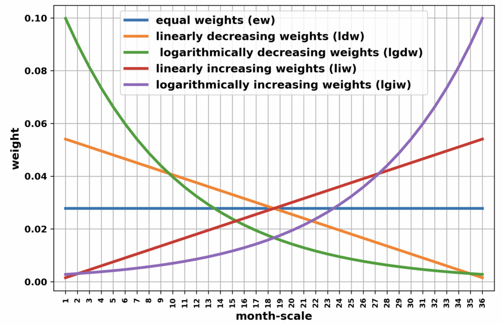
- Equal weights (ew): all SPIs have the same weight (1/n).
- Linearly decreasing weights (ldw): more importance to SPIs on recent time scales, with weights decreasing linearly into the past.
- Linearly increasing weights (liw): the opposite of ldw scheme, giving priority to longer time scales.
- Logarithmically decreasing weights (lgdw): similar to ldw scheme, but with exponential decay, placing even more emphasis on the present.
- Logarithmically increasing weights (lgiw): the opposite of lgdw scheme, with even greater emphasis on the long time scales.
Weights are normalized so that their sum equals 1, and can be applied on a linear or logarithmic basis. The use of weighting allows the index to be adapted to monitoring or risk analysis needs, selecting the function that best aligns with a relevant impact variable (e.g., discharge, damages, etc.).
Overall, strongly negative D(SPI) values represent a clear signal of severe drought conditions, as they indicate multiscale coherence in accumulated precipitation deficits. Conversely, values close to zero or positive correspond to normal water conditions or recovery phases, when the system is progressively rebuilding its reserves.
In the Po river basin, used as first test area, an operational threshold of D(SPI) < –1 was established, capable of consistently identifying all major historical droughts observed from 1960 to the present.
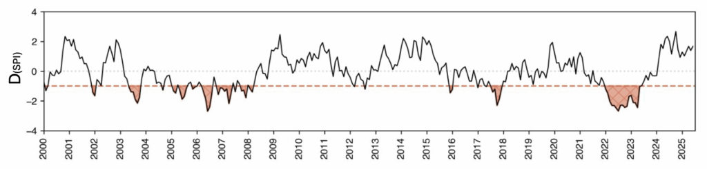
The goal of D(SPI) is to provide a single indicator, calibrated to the basin of interest, capable of highlighting the onset or a possible approach of a severe phase, through a synthetic and objective measure of the event. D(SPI) is also useful as an operational tool for defining alert thresholds, triggering specific conditions in decision models, or supporting management and planning evaluations.
CDN - Cumulative Deviation from Normal
The CDN is the curve of cumulative anomalies of the SPI1 index and can be used to represent the cyclical and multi-year phases of precipitation.
Unlike multiscale indices, which capture conditions up to 36 months, the CDN describes the evolution of the system over longer horizons, highlighting wet phases (positive trends), dry phases (negative trends), or stationary periods, allowing the evaluation of the duration of these cycles. The alternation of these dynamics constitutes the “system memory”, showing how precipitation follows irregular multi-year cycles, which are therefore difficult to predict.
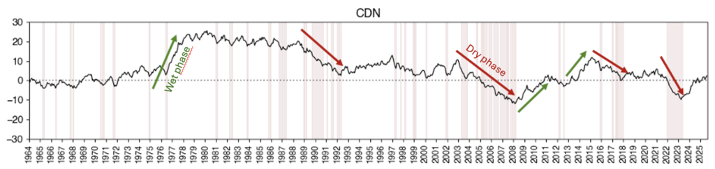
Moreover, the CDN highlights another aspect often overlooked in monitoring systems. The most severe events tend to emerge predominantly at the end of a multi-year downward phase of the CDN. This progressive accumulation of deficit determines the system’s prior exposure and explains why some droughts are more damaging than others, even when the deficit is similar.
NOTE: An additional advantage of CDN is the ability to quantify accumulated surpluses and deficits in terms of millimeters of rainfall. Since SPI1 is a standardized index, the CDN represents the number of cumulative standard deviations, which can be easily converted into millimeters using the standard deviation of precipitation over the reference climatological period. This allows the estimation of water volume lost or gained over a specific period, providing practical support for medium- to long-term water planning and management.
The Drought Scan Seasonal Drought Forecasts
The DS also includes a specific module dedicated to seasonal forecasts with a 1–6 month horizon, combining What-If scenarios with predictions from Earth System Models (ESMs)—global coupled land-ocean-atmosphere models (e.g., the forecasting system of the European Centre for Medium-Range Weather Forecasts, ECMWF).
This module integrates current condition data, thus completing the “historical analysis–monitoring–forecasting” cycle and providing a fully operational climate service.
"What-If" scenarios
The What-If scenarios represent a grid of possible rainfall deficit/surplus evolution based on simple, verifiable probabilistic assumptions. Within the 1–6 month forecast window, different precipitation levels are simulated as multiples or fractions (0.25, 0.50, 0.75, 1.0, 1.25, 1.50, 2.0) of the basin climatology. For each scenario, predicted SPI, D(SPI), and CDN time series are calculated while keeping the statistical distributions of the reference climatological period unchanged.
This approach provides an immediate representation of how the system would react to a given future surplus or deficit of precipitation. In addition, the What-If scenario grid serves as an interpretative tool for analyzing the trajectories traced by seasonal forecasts from the ESMs.
Seasonal forecasts
ESM forecasting systems provide a set of potential future evolutions—the ensemble members—which represent trajectories generated from different initial conditions.
In the DS, precipitation forecasts from the ESM are compared with its internal climatology to derive predicted anomalies. These anomalies are then transformed into 36 SPI values, from which future trajectories of CDN and D(SPI) are subsequently reconstructed.
The result is a range of possible scenarios, represented through the ensemble median and its variability bands (interquartile ranges or standard deviations), providing a clear and effective view of the expected evolution over the coming months.
This approach translates complex model outputs into actionable, interpretable information, integrating meteorological forecasts with real-time monitoring and the meteoclimatic–hydrological continuum already represented by the system.
How to read seasonal forecasts for the D(SPI) index
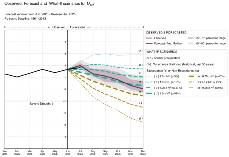
Seasonal forecast of the D(SPI) index obtained from ESM ECMWF forecast, starting in June 2025 for the Po river basin.
- Black line: observed values up to June 2025.
- Purple line: ensemble median of the ESM forecast.
- Shaded bands: interquartile range of the ensemble (indicating the dispersion among members).
- Colored dashed lines: What-If scenarios based on different assumptions of future precipitation. For example: line (d) = normal precipitation; line (a) = double the normal precipitation; line (g) = one-quarter of the normal precipitation.
In the example: the purple line converges between lines (e–d), suggesting that by the end of the semester (February), precipitation conditions are expected to be slightly below average.
P.S.: Working across several river basins, including those outside Italy, the SPI is generally calculated using global precipitation datasets, which may lead to local overestimations or underestimations. From an operational perspective, customized analyses based on proprietary datasets are therefore available upon request, provided that the datasets are sufficiently robust.
Drought Scan in a nutshell
Short videos to explore the context and structure of the climate service
Publications
A. Di Paola, E. Di Giuseppe, R. Magno, S. Quaresima, L. Rocchi, E. Rapisardi, V. Pavan, F. Tornatore, P. Leoni, M. Pasqui. (2025) Building a framework for a synoptic overview of drought. Science of The Total Environment, Vol. 958, 177949. https://doi.org/10.1016/j.scitotenv.2024.177949
Resources
Open source official DS library available at:
- GitHub repository: https://github.com/PyDipa/DroughtScan/tree/main
- PyPI package: https://pypi.org/project/droughtscan/